TASC: Fast Skill Chaining for Complex Sequential Robotic Tasks via Pure Imitation Learning

Abstract

We present TASC: Termination Action Skill Chaining, a method for pure imitation learning of complex sequential long-horizon tasks, requiring only simple sub-task annotations and no environmental reward. We define a new termination action dimension to allow each sub-task’s termination function to be learned jointly with its policy, giving it the ability to end its sub-task. These policies are trained in parallel on segments of the demonstration, and then chained together at inference time, providing a massive speed-up over sequential training. We evaluate TASC on three complex robotic manipulation tasks and show improved success rates compared to state of the art methods.

Keywords: Robotics, Imitation Learning, Skill Chaining, Reinforcement Learning, Option Framework

1 INTRODUCTION

A key challenge in robotics is learning to break up complex tasks into shorter, easier sub-tasks which can be chained together to complete the entire task. Within this scope, we are interested in two key challenges: completing strongly sequential long-horizon tasks, and learning such tasks purely from demonstrations without having to provide an external reward. The combination of these two challenges has received less attention and forms the basis of our work.

We focus on problems where sub-tasks must be completed in a strongly defined order to achieve the final goal, and any failures on the way to the goal become a failure for the entire task. This special case is common in industrial settings such as pharmaceutical robotics, where chemicals must be handled in a specific order in order to facilitate a specific chemical reaction; and manufacturing of building materials, where blocks must be wrapped before they are placed on a pallet. In these fields, safety standards dictate that the robot cannot move onto the next step until it is safe to do so (ISO, 2025).

Many existing approaches solve the general problem of learning tasks with multiple sub-tasks, usually by learning multiple sub-policies and using them at different stages to perform different parts of the task. We demonstrate that many of these approaches do not work well on strongly-sequential long-horizon tasks (see Section 4.4).

We argue that, in order to ensure generality, these approaches rely on one or more of the following implicit assumptions, which make them less suitable for this kind of task:

Figure 1: The Franka Kitchen environment (Gupta et al., 2020), comprising multiple potential sub-tasks such as Kettle, Microwave, Bottom Burner, Top Burner, Slide Cabinet, Hinge Cabinet, Light Switch. In our work, we chain these sub-tasks into long sequences, where all sub-tasks must be completed in order to consider the task successful.

1. One-step option switching: Switching to any sub-policy can be done at any time, meaning that there is no explicit waiting for a termination condition before deciding to change to the next policy. This allows any sub-task to start before the current sub-task is completed.

2. Probabilistic termination: Deciding to switch sub-policies is modelled by a probability distribution, rather than being deterministically based on the current state of the environment. This increases the chance of terminating a subtask early.

3. Order-agnostic completion: The task can still be completed even if the sub-tasks are completed in a different order. This assumption is violated by strongly sequential tasks.

By creating and testing a formulation that challenges these assumptions, we empirically show that none of these algorithms can consistently succeed at strongly sequential long-horizon tasks if they are based on one or more of the above assumptions (see Section 4.4).

When full-task success is important and sub-tasks must be completed in order, we need to revisit these assumptions. We present TASC: Termination Action Skill Chaining, an approach to learning complex sequential long-horizon tasks purely from demonstrations. We define a new action dimension, based on a deterministic version of the dimension introduced in TACO (Shiarlis et al., 2018). This action dimension allows termination deterministically based on the current state (removing Assumption 2, and tested in the ablation study in Section 5), and is learned jointly as a part of each sub-policy. We only allow the sub-policy to transition forwards to the next one when it has reached a fixed sub-task completion confidence threshold $\varphi$ (Section 3.1). We do not allow the sub-policy to transition backwards, or move arbitrarily between sub-policies (removing Assumptions 1 and 3). Our algorithm also performs padding (noise-added zero-padding, Section 3.2) in the demonstration dataset at transition points, which we show improves performance significantly when combined with our deterministic termination indicator. We show that TASC outperforms a variety of baselines (Section 4.4) on three sequential long-horizon robotics domains.

2 RELATED WORK

2.1 Flat IL Methods

Behaviour Cloning (BC) (Bain and Sammut, 1995) is considered the simplest form of IL, where supervised learning is used to learn a policy which maximises the likelihood of generating the provided demonstration dataset. It has been noted that BC struggles with covariate shift (Ross et al., 2011), leading to poor convergence on tasks with multiple sub-tasks.

Diffusion Policy (Chi et al., 2025) is a diffusion-based approach to IL. It focuses on learning a policy through a conditional denoising diffusion process. Chi et al. report good results for DP on long-horizon tasks with multiple sub-tasks, such as those within the Franka Kitchen environment. It must be noted, however, that this is only true when the action-space of Franka Kitchen has been altered to be position-based, which Chi et al. do in their original paper, as they state that DP can struggle with velocity-based action spaces. We do not implement such changes, which we explain further in Section 4.4.

2.2 Hierarchical Methods

A number of approaches address learning multi-step tasks by imposing some form of task hierarchy. Some approaches focus on learning reusable sub-policies that can be chained together in different forms to attempt to complete multiple tasks (Sharma et al., 2019; Jing et al., 2021; Chen et al., 2023; Qiu et al., 2024). Other methods focus on solving a single task, with strongly sequential skill-chaining of multiple sub-policies (Jain and Unhelkar, 2024; Sharma et al., 2019; Shiarlis et al., 2018).

2.2.1 Multi-task Hierarchical IL

Multi-task hierarchical IL is a learning paradigm based on the idea that different, related tasks have sub-tasks in common. This means that sub-tasks only need to be learned once, and then reused for different tasks. Some methods perform multi-task hierarchical IL on long-horizon tasks such as those within the Franka Kitchen environment (Gupta et al., 2020), but require live samples through environment interaction during training. On simpler singular tasks such as the CloseMicrowave2 task (Jing et al., 2021), they converge poorly.

EM-based methods are the most common approach within multi-task HIL, simultaneously learning low-level sub-policies and a high-level meta controller, often from unsegmented demonstrations. This is done by estimating the options during the E-step and updating the policies and options during the M-step (Chen et al., 2023; Jing et al., 2021).

Within the special case of learning strongly-sequential long-horizon tasks, we believe that success rates are more interesting than reward. A high reward may still hide the fact that there has been a catastrophic failure in one of the sub-tasks; e.g. the agent continues to accrue high reward because it is physically close to the goal, but it has let go of the object. A high success rate has no such ambiguity.

We test these EM-based approaches on single long-horizon tasks within Franka Kitchen and other environments in Section 4. In our testing, these methods did not reliably complete the entire task.

The methods outlined in this section make two core assumptions:

• They are based on the one-step option paradigm (Assumpton 1), meaning that the high-level policy can select a new sub-policy at any time conditioned on the current state.

• They also assume order-agnostic completion (Assumption 3), the idea that sub-tasks can be completed in any order, rather than in a specific sequence. This likely contributes to low success rates, compared to their higher reward. We test both in Section 4.

2.2.2 Single-task IL with Skill Chaining

Skill-chaining approaches designed specifically for single-task IL include:

GO-DICE (Jain and Unhelkar, 2024) learns a multi-step task from unsegmented demonstrations by using stationary distribution correction estimation (DICE) to train a high-level policy and a set of low-level policies. It introduces multi-fetch versions of sequential pick and place tasks (PnP$\times 2$ and PnP$\times 3$, covered further in Section 4). GO-DICE does not report full-task success rates, but does report strong rewards for standard Fetch PnP$\times 1$ (Plappert et al., 2018), PnP$\times 2$ and PnP$\times 3$.

DI-GAIL (Sharma et al., 2019) approaches option learning from unsegmented demonstrations by maximising directed information flow through a series of latent variables representing the task context, and learning sub-policies with GAIL (Ho and Ermon, 2016) based on a prior distribution of latent variables learned by a VAE (Kingma and Welling, 2014). DI-GAIL is successful in simpler gym domains but requires further reward engineering to substantially improve the reward of the Fetch PnP$\times 1$ task over traditional end-to-end IL methods.

TACO (Shiarlis et al., 2018) learns a multi-step task by using temporal alignment to transform unsegmented demonstrations including task-sketch information into segmented demonstrations, and then uses these to learn a set of sub-policies. One of the methods introduced as a supervised baseline in this paper is GT-BC, and our work is based on its underlying formulation. TACO and GT-BC both make the probabilistic termination assumption (Assumption 2), meaning that there is always randomness inherent in deciding termination, rather than being deterministically based on the state. We base our approach on GT-BC, but make the following changes:

1. Deterministic Termination Indicator:
   Our approach uses a deterministic termination indicator based on a threshold instead of a probability, designed to match the strongly sequential aspect of these tasks. This is explained further in Section 3.1.

2. Noise-added Zero-padding:
   Our approach also includes a pre-processing step which applies noise-added zero-padding on the transition points, based on some easily defined state and action identity functions $I_S(s)$ and $I_A(a)$, explained further in Section 3.2.

Our experiments confirm the importance of these changes, showing that TASC significantly outperforms GT-BC on all baselines (Table 1). We also test the importance of each of these changes in the ablation study in Section 5.

3 TERMINATION ACTION SKILL CHAINING (TASC)

3.1 Problem Formulation

Given a dataset with labelled transition points, we do the following to learn each sub-task $h\in \mathscr{H}$ and termination function $B$. In our experiments, we assume that only the timestamps for transition points are given (further explained in Section 1).

Deterministic Policy:

For inference, each sub-task’s policy ${\mu }_h$ can be represented as a deterministic mapping from the current state $s$ to the action $a$ and termination indicator $\beta$ (the realisation of the termination function $B$). This allows the computation of of $a$ and $\beta$, given a state $s$, as follows:

$(a,\beta )\leftarrow {\mu }_h(s),$ (1)

where the output of ${\mu }_h(s)$ here refers to the mean/mode of the trained Gaussian policy, based on the following formulation:

${\pi }_h(\cdot |s)=𝒩({\mu }_h(s),{\sigma }_h{(s)}^2),$ (2)

where $𝒩(\mu ,{\sigma }^2)$ is the Gaussian distribution with mean $\mu$ and standard deviation $\sigma$.

In practice, allowing $\beta$ to be generated by ${\mu }_h$ is done by introducing a new dimension to the action to be learned by the policy (Barreto et al., 2019; Shiarlis et al., 2018). We base our termination indicator $\beta$ on the $a_{STOP}$ action dimension introduced in TACO (Shiarlis et al., 2018).

Algorithm 1 TASC: Termination Action Skill Chaining (Training Process)

Input: Demonstration dataset ${𝒟}^{\prime }$ List of transition points for each trajectory ${\mathrm{\Psi }}_{\tau }=\{0,{\psi }_1,\mathrm{\dots },{\psi }_N\}$ Learning rate $\alpha$

Use Equations 9 and 10 to get ${𝒟}^{\ast }$ from ${𝒟}^{\prime }$ with $I_A^{\prime }(a)$ and $I_S^{\prime }(s)$

$N\leftarrow |{\mathrm{\Psi }}_{\tau }|-1$ $▷$Get number of sub-tasks from transition point list

for $h\leftarrow 0$ to $N-1$ do  $▷$For each sub-task (in parallel)

     Initialise feed-forward Gaussian policy network ${\pi }_h^{\theta }$ with random weights

     repeat until convergence  

      Sample $(s,a,\beta )\sim {𝒟}_h^{\ast }$

      Compute $ℒ(\theta )=-log{\pi }_h^{\theta }(s,a,\beta )$

      Update $\theta \leftarrow \alpha {\nabla }_{\theta }ℒ(\theta )$

     end repeat

end for

Deterministic Termination Indicator:

We allow the agent to terminate the current episode based on the termination indicator $\beta$ during inference, when the condition $\beta \ge \varphi$ is satisfied, where $\varphi$ is the termination threshold defined as a hyperparameter. We start with a demonstration dataset $𝒟$:

$𝒟={\{{\tau }^{(i)}\}}_{i=0}^M,$ (3)

where $M$ is the number of demonstrations. Each demonstration $\tau$ is represented as:

$\tau ={\{(s_t,a_t)\}}_{t=0}^T,$ (4)

where T is the length of the demonstration in timesteps. We also accept a list of transition points ${\mathrm{\Psi }}_{\tau }$ for each trajectory $\tau$:

${\mathrm{\Psi }}_{\tau }=\{0,{\psi }_1,\mathrm{\dots },{\psi }_N\},$ (5)

where $N$ is the number of sub-tasks, ${\psi }_h$ is the index of the transition point from sub-task $h$ to $h+1$, and ${\psi }_0=0$ represents the initial state for convenience.

An augmented dataset ${𝒟}^{\prime }={\{{\tau }^{\prime (i)}\}}_{i=0}^M$ can be created to contain the transition points represented as termination indicator $\beta =1$. ${𝒟}^{\prime }$ contains demonstrations ${\tau }^{\prime }$:

${\tau }^{\prime }={\{(s_t,a_t,{\beta }_t)\}}_{t=0}^T,$ (6)

where ${\beta }_t$ is the termination indicator at time $t$.

The same trajectory ${\tau }^{\prime }$ can be split into sub-trajectories ${\tau }_h^{\prime }$ and filled with ground truth values for the termination indicator $\beta$, where the transition points are given by ${\mathrm{\Psi }}_{\tau }$:

${\tau }_h^{\prime }={\{(s_t,a_t,-1)\}}_{t={\psi }_{(h-1)}}^{({\psi }_h)-1},(s_{{\psi }_h},a_{{\psi }_h},1);$ (7)

where $h$ is the sub-task, and $t$ is the current timestep. Non-transition points are represented by a termination indicator of $\beta =-1$.

3.2 Training TASC

To train a TASC agent (Algorithm 1), the demonstrations are processed to fit the formulation in Section 3.1. In practice, we must also pad each trajectory with repeated steady states at all transition points, so the termination indicator $\beta$ has a balanced number of positive and negative examples. We show that this increases performance significantly in the ablation study (Section 5). These steady states (and zero-actions) are calculated based on the following:

For an action $a$, $I_A(a)$ is defined as the action which attempts to keep environment in the same state regardless of how many times $I_A(a)$ is applied. Given a previous state $s$, $I_S(s)$ outputs the state that assumes there is no movement since the previous state $s$. These identity functions are easily created based on the action space and state space of the environment, and need only be defined once per environment.

Noise-added Zero-padding:

In practice, we use a noisy identity function in place of the standard identity function to inject a small amount of uniform noise, to help expand coverage of the state space and action space at the transition point, instead of repeating the exact same state-action pair. This noisy identity distribution $I^{\prime }(s)$ can be sampled from in place of the identity function $I(x)$ and is defined as follows:

$I^{\prime }(x)=I(x)+𝒰(x-ϵ,x+ϵ),$ (8)

where $𝒰(x,y)$ a uniform distribution of real numbers in the range $[x,y]$, so $ϵ$ gives the noise range. A padded sub-trajectory can be obtained by padding with identity actions and identity states at each termination point, doubling the final size of the sub-trajectory:

${\tau }_h^{\ast }=$ ${\{(s_t,a_t,0)\}}_{t=2{\psi }_{(h-1)}}^{({\psi }_h)-1},$ (9)

${\{(s\sim I_S^{\prime }(s_{{\psi }_h}),a\sim I_A^{\prime }(a_{{\psi }_h}),1)\}}_{t={\psi }_h}^{2{\psi }_h};$

where $N$ is the number of sub-tasks, $h$ is the current sub-task, and $t$ is the current timestep. Each sub-task policy will be trained on a dataset of sub-trajectories corresponding to the sub-task index $h$. In full, sub-task $h$ will be trained on all trajectories corresponding to ${𝒟}_h^{\ast }$:

${𝒟}_h^{\ast }={\{{\tau }_h^{\ast (i)}\}}_{i=0}^M,$ (10)

where $h$ is the sub-task index to train, and $M$ is the number of trajectories.

The list of transition points ${\mathrm{\Psi }}_{\tau }$ defined in Equation 5, gives the ascending list of indices $(0,{\psi }_1,\mathrm{\dots },{\psi }_N)$ of the sub-task transition points (including 0, to represent the start point of the first sub-task).

As highlighted in Algorithm 1, given these datasets the policies can be trained separately. No information is shared between them, so they can be trained in parallel. For each sub-task index $h$, training is completed for a set number of training steps $M$.

A feed-forward Gaussian policy network ${\pi }_h^{\theta }$ is initialised with random weights $\theta$ for each sub-task $h$. At each time-step a state, action, termination indicator tuple is sampled uniformly from the dataset:

$(s,a,\beta )\sim {𝒟}_h^{\ast },$ (11)

where ${𝒟}_h^{\ast }$ is sampled from to obtain a random $(s,a,\beta )$ sample from the demonstration dataset ${𝒟}_h^{\ast }$. The negative log-likelihood loss is computed on this tuple, based on the Gaussian policy used during training:

$ℒ(\theta )=-log{\pi }_h^{\theta }(s,a,\beta ).$ (12)

The NLL loss is then used to update the policy parameters $\theta$:

$\theta \leftarrow \alpha {\nabla }_{\theta }ℒ(\theta ).$ (13)

After training every sub-task $h$ in parallel, a list of Gaussian policies $({\pi }_0,{\pi }_1,\mathrm{\dots },{\pi }_{N-1})$ will exist whose deterministic counterparts $({\mu }_0,{\mu }_1,\mathrm{\dots },{\mu }_{N-1})$ can be used sequentially for deterministic inference at runtime. The segment of the demonstration dataset used to train each sub-task is completely separate, and no data is shared between sub-policies during training. This means that the policies can be trained fully in parallel on separate cores, speeding up the training by up to a factor of $N$ (where $N$ is the number of sub-tasks) when compared to sequential training.

4 EXPERIMENTAL SETUP AND RESULTS

4.1 Environments

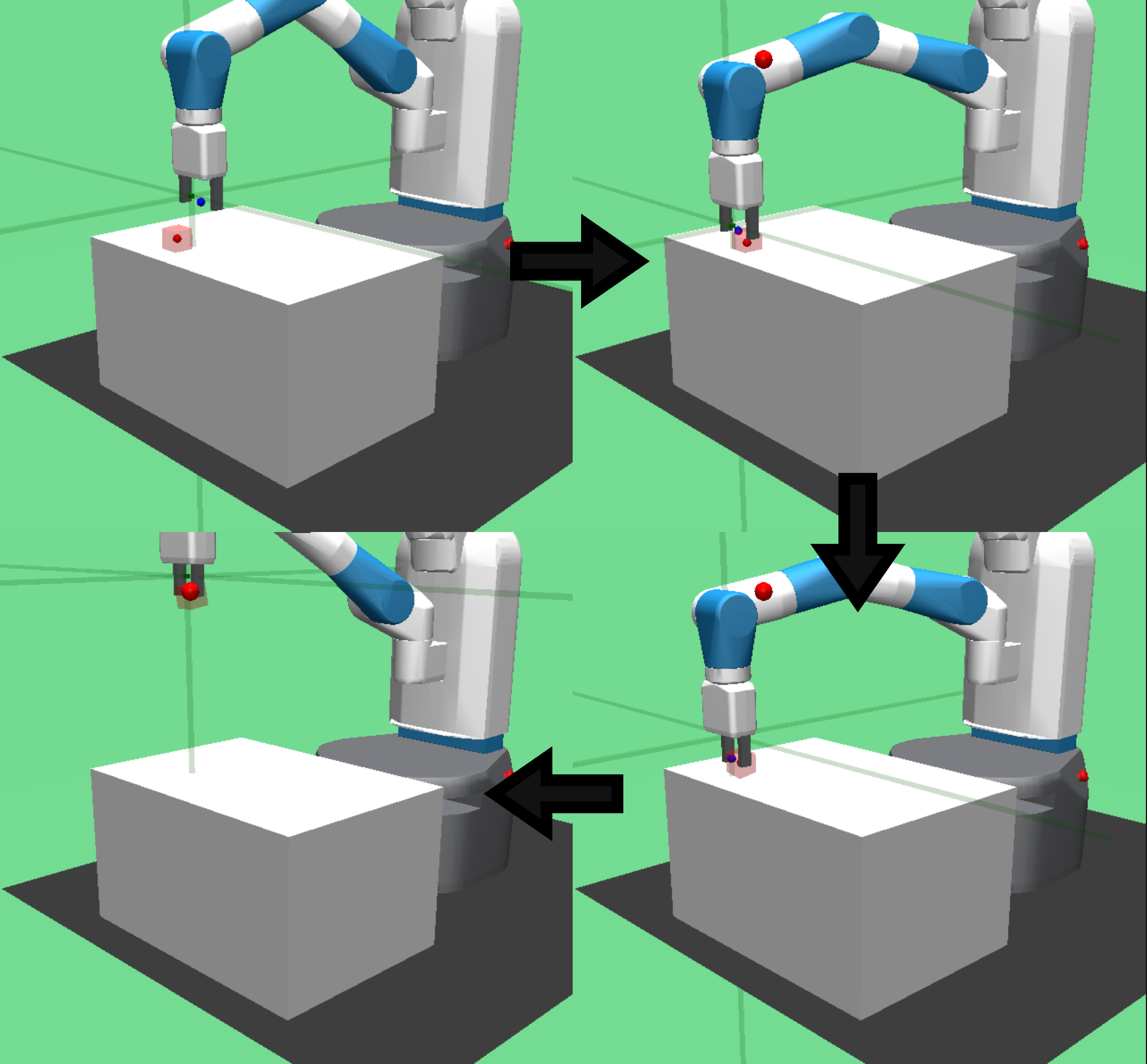
Fetch (Figure 3) was chosen as an environment due to its multi-step nature and strong variability, where its pick and place task (PnP$\times 1$) has a uniformly sampled initial object position and target position. The goal is to bring the object to the target within a threshold of 0.05m. It is clear that the sub-tasks determined by the transition points in Section 1 and in Figure 3 must be done in the correct order (see Assumption 3).

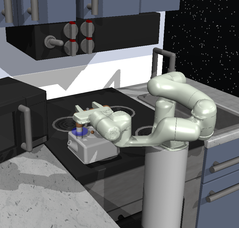
Franka Kitchen (Figure 1) was chosen due to its popularity as an evaluation environment for long-horizon tasks, and due to its richer interaction with multiple different types of object. A success signal is given at the end when all objects are within 0.3 units of their targets. Our main experiments (summarised in Table 1) use a pre-segmented demonstration dataset on the following macro sub-tasks: Kettle, Microwave, Slide Cabinet, which we split into further sub-tasks.

The demonstrations only contain the sub-tasks in one order, removing the order-agnostic completion assumption (Assumption 3).

Figure 2: The MultiFetch environment (PnP$\times 2$) (Plappert et al., 2018; Jain and Unhelkar, 2024). The objects are both randomly placed on the table, and must be brought to their respective randomly positioned targets on the table.

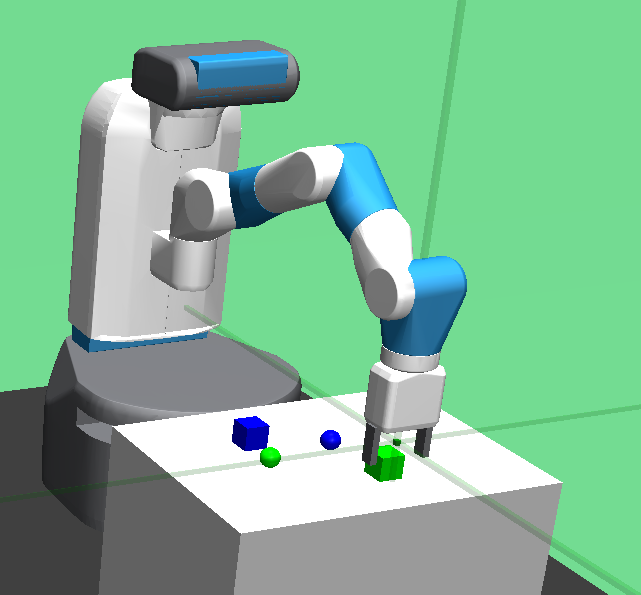
MultiFetch was chosen to test both variability and complexity, where the task is the same as Fetch (PnP$\times 1$), but with 2 objects (PnP$\times 2$), and targets are placed on the table instead of in the air. As introduced by GO-DICE (Jain and Unhelkar, 2024), PnP$\times 2$ consists of 2 objects whose initial positions and target positions are both uniformly sampled from the space. As with PnP$\times 1$, the goal is to bring both objects to their respective targets within a threshold of 0.05m.

4.2 Algorithms

To test against a wide range of methods, we chose approaches from the single-task and multi-task paradigms (provided with pre-segmented demonstrations for a fair comparison), and also two flat IL algorithms. In order of presentation in Table 1, the algorithms tested are:

Flat IL algorithms:

BC (Behaviour Cloning) (Bain and Sammut, 1995). BC is tested due its popularity as the simplest IL algorithm. DP-C (Diffusion Policy-CNN) (Chi et al., 2025). DP is tested due to its popularity as a new technique which has strong results on a variety of robotic tasks, including those in the real-world. (Chi et al., 2025) report that velocity-based action spaces are not as easily solvable by DP, and in the case of the Franka Kitchen environment, reduce the final success rate by as much as 100% (this can be observed in Table 1).

Multi-task algorithms (one-step option):

OptionGAIL (Adversarial Option-Aware Hierarchical Imitation Learning) (Jing et al., 2021) is a well known baseline which many EM-based methods within multi-task IL build upon. MH-AIRL (Multi-task Hierarchical Adversarial Inverse Reinforcement Learning) (Chen et al., 2023) is an improvement on OptionGAIL using AIRL rather than GAIL. SeqNMF (Sequential Non-negative Matrix Factorisation) (Qiu et al., 2024) is a more recent method which uses non-negative matrix factorisation to learn multiple tasks.

Single-task algorithms (including skill chaining):

DI-GAIL (Directed-Info GAIL) (Sharma et al., 2019) was chosen due to its position as a well-known baseline for sequential option learning. GO-DICE (Goal-Conditioned Option-Aware Offline Imitation Learning via Stationary Distribution Correction Estimation) (Jain and Unhelkar, 2024) was chosen as it reports good results on the Fetch task and introduces the MultiFetch setting. GT-BC (Ground Truth Behaviour Cloning) (Shiarlis et al., 2018) was chosen for comparison as it is the foundation for TASC.

Our approach:

TASC (Termination Action Skill Chaining). Explained in detail in Section 3.1 and Section 3.2.

4.3 Transition Point Labelling

Figure 3: The labelling regime used to label all demonstration transition points. The example shows the Fetch PnP$\times 1$ task (Plappert et al., 2018). Top-left: the start point (${\psi }_0$). Top-right: the object is found (${\psi }_1$). Bottom-right: the object has been grasped (${\psi }_2$). Bottom-left: the object has been taken to the target (not a transition point, but the success state of the environment, used only in evaluation).

Table 1: Evaluation reward and full-task success rate for selected algorithms. Every algorithm (aside from BC and DP-C) is provided with pre-segmented demonstrations for a fair comparison. The results are much more close when comparing the evaluation reward, as suspected, as TASC (ours) was specifically designed to be focused on maximising success rate rather than reward. Each algorithm was provided with 200 demonstrations of each task.

Algorithm	Steps	Fetch (PnP$\times 1$)		MultiFetch (PnP$\times 2$)		Franka Kitchen
		Reward	Succ.	Reward	Succ.	Reward	Succ.
BC (Bain and Sammut, 1995)	$5\times {10}^5$	$-0.093$	$0.76$	$0.435$	$0.03$	$123.5$	$0.04$
DP-C (Chi et al., 2025)	$1\times {10}^5$	$-0.325$	$0.01$	$0.400$	$0.01$	$10.53$	$0.00$
OptionGAIL (Jing et al., 2021)	$8\times {10}^6$	$-0.314$	$0.01$	$0.275$	$0.00$	$0.000$	$0.00$
H-AIRL (Chen et al., 2023)	$8\times {10}^6$	$-0.312$	$0.01$	$0.250$	$0.01$	$0.000$	$0.00$
SeqNMF (Qiu et al., 2024)	$8\times {10}^6$	$-0.321$	$0.01$	$0.251$	$0.00$	$0.000$	$0.00$
DI-GAIL (Sharma et al., 2019)	$8\times {10}^6$	$-0.282$	$0.00$	$0.246$	$0.01$	$92.59$	$0.00$
GO-DICE (Jain and Unhelkar, 2024)	$1\times {10}^5$	$-0.151$	$0.58$	$0.290$	$0.00$	$88.00$	$0.00$
GT-BC (Shiarlis et al., 2018)	$5\times {10}^5$	$-0.324$	$0.25$	$1.560$	$0.15$	$100.5$	$0.00$
TASC (ours)	$5\times {10}^5$	$-\mathbf{0.084}$	$\mathbf{0.90}$	$\mathbf{1.655}$	$\mathbf{0.35}$	$\mathbf{252.5}$	$\mathbf{0.76}$

To ensure the best possible demonstrations for all algorithms, we trained a SAC synthetic expert and used an oracle to label transition points (used in Section 3.1, specifically Equation 5). In real deployment, these would be replaced by VR demonstrations, and transition point labelling would be carried out during VR demonstration collection with minimal extra effort, e.g. by pressing a button at each transition point. Methods also exist to obtain these automatically from unsegmented demonstrations (Krishnan et al., 2017; Zhang et al., 2024).

4.4 Results

The algorithms from Section 4.2 are run on the environments from Section 4.1, with results shown in Table 1, which shows the full-task evaluation success rate and reward. TASC outperforms all of the baselines in terms of full-task success rate when all are provided with pre-segmented demonstrations. The results are much closer when comparing against the evaluation reward, which makes sense when considering that TASC was designed with sequential full-task success in mind, rather than reward.

Although TASC is based on the GT-BC approach outlined in TACO (Shiarlis et al., 2018), GT-BC does significantly worse across all environments compared to TASC. GO-DICE outperforms GT-BC on Fetch (PnP$\times 1$), but not BC. BC likely performs well as (PnP$\times 1$) is the shortest-horizon of the tasks tested.

DP-C (Diffusion Policy-CNN) has low success rates across all tasks, but this is likely because the environments are all within a velocity-based action space. Chi et al. report that in the Franka Kitchen environment, there is an average of an 100% success rate increase (i.e. from 0.0 to 1.0) when engineering the environment to switch from a velocity-based action space to a position-based action space. For fairness across algorithms, and as velocity-based action spaces are much more common and more conducive to Sim2Real transfer (Höfer et al., 2021) than position-based on manipulation tasks (Aljalbout et al., 2024), we leave this analysis for future work.

Multi-task algorithms (OptionGAIL, H-AIRL, SeqNMF) do significantly worse than the single-task algorithms, likely due to being designed to solve a different problem. Multi-task learning is a more difficult problem, but requires a different set of assumptions, so methods specific to multi-task learning are not necessarily good at single-task learning, especially in longer-horizon sequential domains.

The demonstrations also contain a finer sub-task granularity, and only of a single task (although the number of demonstrations is higher). This compares to the demonstration dataset used by the multi-task baselines (Jing et al., 2021; Chen et al., 2023; Qiu et al., 2024), where unsegmented demonstrations from multiple different tasks are used (labelled with rough task sketches).

Table 2: Evaluation reward and full task success rates for Franka Kitchen (Kettle, Bottom Burner, Light Switch, Hinge Cabinet). 20 unsegmented demonstrations of multiple different tasks are provided, better fitting the assumptions made by these algorithms. Results are better under these conditions, even with fewer demonstrations.

Algorithm	Franka Kitchen
	Reward	Succ.
OptionGAIL (Jing et al., 2021)	94	0.00
H-AIRL (Chen et al., 2023)	88	0.00
SeqNMF (Qiu et al., 2024)	204	0.02

The formulation for these methods assumes that this kind of variety is provided, which could explain why they perform worse when only given finer, pre-segmented demonstrations of a single long task, as this breaks their assumptions. To test this, we run an extra set of experiments using the dataset provided on the following set of sub-tasks: Kettle, Bottom Burner, Light Switch, Hinge Cabinet. This experiment, shown in Table 2, shows that even when the dataset is set up for the assumptions made in the multi-task approaches (Jing et al., 2021; Chen et al., 2023; Qiu et al., 2024), this does not translate to a high success rate. Although high rewards can be accrued, success rates do not necessarily follow, as if any intermediate sub-tasks are missed, the final success rate will be 0.

5 ABLATION STUDY

Table 3: Ablation study for full task success rates of GT-BC vs TASC on Fetch for 500k steps. We test the two changes made to GT-BC in creation of TASC. Both changes increase the performance of GT-BC, but achieve the best result when combined together. Table 1 shows the same outperformance of TASC over GT-BC on multiple tasks.

Algorithm	Fetch (Succ.)
GT-BC (Shiarlis et al., 2018)	0.25
GT-BC - deterministic termination only	0.70
GT-BC - noise-added zero-padding only	0.83
TASC (ours)	0.90

In this ablation study (Table 3), we test the two additions to GT-BC separately, and show that they are both required. Vanilla GT-BC (probabilistic termination, no padding) was the lowest performer, but showed significant improvement from 0.25 to 0.7 when adding the deterministic termination indicator. If noise-added zero-padding was added instead, the performance improved further up to 0.83. When both are added together, this is the formulation for TASC. It performs best at 0.9, suggesting that both changes (covered in Sections 3.1 and 3.2) are required.

6 CONCLUSION

We introduce TASC (Termination Action Skill Chaining), a method for learning long-horizon, strongly sequential tasks from pre-segmented demonstrations. We highlight three assumptions that are widely made within the literature: One-step option switching (Assumption 1), probabilistic termination (Assumption 2), and order-agnostic completion (Assumption 3). We define a method which challenges the above, based on sequential sub-policy switching with a deterministic termination indicator and adding noise-based zero-padding. We show empirically that challenging these assumptions allows our method to outperform strong baselines in the literature in the case of strongly-sequential robotic tasks, when all methods are provided with pre-segmented demonstrations. Our method will not outperform more general algorithms on more general tasks, but does perform better on this subset of the problem space.

7 FUTURE WORK

TASC learns long-horizon strongly sequential tasks given transition points, however relying on transition points is less desirable than learning from unsegmented demonstrations. Future work into learning from unsegmented demonstrations could aim to combine the formulation presented with a joint approach to sub-task discovery and chaining, or a decoupled approach for automatic segmentation. TASC could also be combined with architectures that allow other state-spaces such as visual input, as many of the real-life use-cases cannot provide state-based information.